Every week, I get the This Week in Rust newsletter to keep up on news in the community. I love reading the blogposts, which always have lots of cool info about various things I don’t know much about in Rust. In the last newsletter, I read an interesting post about why languages become popular and it piqued my interst in Julia, a language I’ve heard of but never used. From what I know, Julia is good at manipulating data and is kinda like MatLab and Python and R. I’ve used MatLab in classes and I have some experience with Python and R for data-science/AI, but I’m not really good at any of them. After looking at Julia’s homepage, I decided to try it out and see what I could learn.
After installing Julia (brew cask install Julia, with homebrew on macOS), I started a Jupyter notebook with a Julia kernel.
julia> import Pkg; Pkg.add("IJulia")
julia> using IJulia
julia> notebook()
Some of the tutorials I found suggested the VSCode Julia extension, and older ones suggested the Atom extension, but I really enjoy the experience of working in a Jupyter notebook. It feels like the best of both worlds from writing scripts and using a REPL: I can try one-off things and inspect values in the middle of the notebook, but I can also write long bits of code and run them together.
Since the Jupyter notebook has markdown cells, I started typing out what I was doing as a roadmap for myself. Eventually, I decided that I might as well make it into a blogpost. In other words, this is a lightly-edited path through my actual experience using Julia for the first time. Most of the content was actually typed while trying out the code.
Let’s get started!
Playing with matrices from \(GL(2, 2)\)
I’ve heard that Julia is a good language for matrix manipulation. Let’s start our exploration by defining some matrices and printing them.
e = [1 0; 0 1]
A = [1 1; 1 0]
B = [0 1; 1 0]

display(e);
display(A);
display(B);
2×2 Array{Int64,2}:
    1  0
    0  1

2×2 Array{Int64,2}:
    1  1
    1  0

2×2 Array{Int64,2}:
    0  1
    1  0
As you can see, the syntax for all of this is pretty standard. While I don’t know what much of this means yet, it seems to be working so far.
You may be asking why I chose to define these relatively simple matrices. The matrices \(e\), \(A\), and \(B\) are from the \(GL(2, 2)\) group, which consists of all of the 2x2 matrices with entries of 1 or 0 and a determinant that isn’t 0. I’m in the middle of learning about \(GL(2, 2)\) in my math course this semester, so I thought it would be a good place to start. Fascinatingly, these three elements can generate the entire group through multiplication. I bet there’s an easier way to do this, but here goes.
GL22 = [e, A, A^2, B, A*B, A^2*B]
6-element Array{Array{Int64,2},1}:
    [1 0; 0 1]
    [1 1; 1 0]
    [2 1; 1 1]
    [0 1; 1 0]
    [1 1; 0 1]
    [1 2; 1 1]
Here, we made an array named GL22 with entries that are other arrays: the matrices in the group.
At the top of the past two outputs, you can see the type of what we’ve made so far.
So we’ve got our group! I mean, as long as you interpret 2s as 0s, since I haven’t taken any modulos. Every element of the group is supposed to only have entries of either 0 or 1. If you multiply a matrix by another and some entry is not 0 or 1, you’re supposed to replace that entry with its mod 2 equivalent. However, I don’t really know how to do that yet, so we’re going to ignore it (for now).
I know from my class that \(A \in GL(2, 2)\) has an order of 3. In other words, \(A^3 = e\), the identity matrix. Let’s try it.
A^3 == e
false
Hmm, okay. I suspect this has something to do with modulo problems. Let’s inspect each side.
println(A^3, " =?= ", e)
[3 2; 2 1] =?= [1 0; 0 1]
Yep, look at that. What happens if I try to take the modulo of a matrix?
A^3 % 2
MethodError: no method matching rem(::Array{Int64,2}, ::Int64)
Closest candidates are: *snip*
Hm… okay. That isn’t helpful. Apparently the naive way doesn’t work. Let’s look up element-wise operations.
According to those docs, element-wise operations just require a dot before the actual operator.
A^3 .% 2
2×2 Array{Int64,2}:
    1  0
    0  1
Woohoo! That worked great. And look, it’s the identity!
(A^3 .% 2) == e
true
Okay, so how can I better define \(GL(2, 2)\)? Is there a way that I can perform the modulo on it implicitly in every multiplication? Or maybe…
GL22 .% 2
MethodError: no method matching rem(::Array{Int64,2}, ::Int64)
Closest candidates are: *snip*
Nope, apparently I can’t apply a modulo through two levels of matrices. Maybe I can iterate over the entries, though?
for M in GL22
    println(M .% 2)
end
[1 0; 0 1]
[1 1; 1 0]
[0 1; 1 1]
[0 1; 1 0]
[1 1; 0 1]
[1 0; 1 1]
Okay, that lets us print the proper, modulo’d matrices. Is there any way to store those, though? And still, we’ll continue to run into the problem where \(A^3 \not= e\) in the code even though it really is.
I know that Julia is a language with inheritance, or at least some sort of subtyping. Maybe I can make my own version of a matrix that always does multiplication modulo 2? Or maybe even multiplication modulo \(n\). I’ll table that for now (there seems to be an interesting package named nemo that might help).
Moving on, every matrix in \(GL(2, 2)\) has a non-zero determinant. Can we calculate the determinants of the matrices we have?
using LinearAlgebra

println("det A = ", mod(det(A), 2))
println("det B = ", mod(det(B), 2))
det A = 1.0
det B = 1.0
That works pretty well. I had to import the LinearAlgebra package in order to use the determinant function, which I found in Julia’s documentation.
If you’re curious why I’m not just using det(A) % 2, it’s because that gives me a negative modulus when I want a positive modulus. For example:
println("(%)    6 % 10 =  ", 6 % 10)
println("(mod)  6 % 10 =  ", mod(6, 10))
println("(%)   -6 % 10 = ", -6 % 10, "   wrong")
println("(mod) -6 % 10 =  ", mod(-6, 10), "   correct!")
(%)    6 % 10 =  6
(mod)  6 % 10 =  6
(%)   -6 % 10 = -6   wrong
(mod) -6 % 10 =  4   correct!
I can only think of one more thing to do with this group: build a multiplication table. Let’s try to write a function that will compute and store the multiplication table for any group given an array that contains every element of that group.
function multable(group::Vector{Matrix{Int64}}, modulo::Int)
    table = Matrix{Matrix{Int64}}(undef, size(group, 1), size(group, 1));
    for (i, X) in enumerate(group)
        for (j, Y) in enumerate(group)
            table[i, j] = (X*Y) .% modulo
        end
    end
    return table
end;
Let’s walk through this function one step at a time. I’m pretty sure it isn’t idiomatic Julia code, since it’s the first Julia function I’ve ever written. Still, it was helpful for me to try.
First of all, the function takes two parameters: group and modulo.
The first of these has type Vector{Matrix{Int64}}, which is just a fancy way of saying a one-dimensional list of two-dimensional objects that contain integers.
If we wanted to be general, we could say that the matrix entries must be elements of a field, but I haven’t actually gotten to that part of my course yet.
The second variable, modulo, has type Int, which means it’s just an integer value.
That’s because we want to take the element-wise modulo of each multiplication’s result, but we don’t know which modulo to take from the group itself.
Next, on line 2, we define our table, which will hold the results of our multiplications.
This was the hardest line for me to write because it required a lot of knowledge of Julia in order to figure out.
The Matrix{Matrix{Int64}}(...) syntax is how you initialize a new matrix of a particular size in Julia. In this case, we’re building a multiplication table, so it must the same number of rows and columns as the number of group elements.
In the case of \(GL(2, 2)\), that’s 6.
We can find out how many elements are in the group by looking at the first dimension of the group vector we’re given. That’s what size(group, 1) does.
As an aside, apparently Julia indexes arrays starting with 1 instead of 0. I can’t remember if MatLab does this, but it strikes me as very odd.
Then, we initialize the table with undef values.
For example, check out what we get from just that line run alone:
group = GL22;
Matrix{Matrix{Int64}}(undef, size(group, 1), size(group, 1))
6×6 Array{Array{Int64,2},2}:
    #undef  #undef  #undef  #undef  #undef  #undef
    #undef  #undef  #undef  #undef  #undef  #undef
    #undef  #undef  #undef  #undef  #undef  #undef
    #undef  #undef  #undef  #undef  #undef  #undef
    #undef  #undef  #undef  #undef  #undef  #undef
    #undef  #undef  #undef  #undef  #undef  #undef
Since \(GL(2, 2)\) has 6 elements, we get a 6x6 table. Theoretically, we could define a group (like \(D_6\) or something) that has more elements and we’d get a bigger table. However, this is all we have so far.
Let’s get back to the function at hand and finish explaining how it works.
Lines 3 through 7 are just two nested for loops, but there are a few interesting things I want to highlight.
First of all, Julia has interation a little bit like Rust, which is the language I’m most comfortable in.
When you write for (i, X) in enumerate(group), Julia gives you the element itself in X and the index of that element in i.
That’s useful for assignment later on because we need to know where in the table our multiplication should go.
Finally, there’s the kicker of the function: table[i, j] = X*Y .% modulo.
Here, we mutate the table we defined earlier, inserting our multiplications into the right spots.
As before, we do the matrix multiplication (X*Y) first and then take the element-wise modulo (.% modulo).
After that, our function is done and we can return the multiplication table!
Let’s give it a whirl.
multable(GL22, 2) # Generate the multiplication table of the GL(2, 2) group, taking each operation modulo 2
6×6 Array{Array{Int64,2},2}:
    [1 0; 0 1]  [1 1; 1 0]  [0 1; 1 1]  [0 1; 1 0]  [1 1; 0 1]  [1 0; 1 1]
    [1 1; 1 0]  [0 1; 1 1]  [1 0; 0 1]  [1 1; 0 1]  [1 0; 1 1]  [0 1; 1 0]
    [0 1; 1 1]  [1 0; 0 1]  [1 1; 1 0]  [1 0; 1 1]  [0 1; 1 0]  [1 1; 0 1]
    [0 1; 1 0]  [1 0; 1 1]  [1 1; 0 1]  [1 0; 0 1]  [0 1; 1 1]  [1 1; 1 0]
    [1 1; 0 1]  [0 1; 1 0]  [1 0; 1 1]  [1 1; 1 0]  [1 0; 0 1]  [0 1; 1 1]
    [1 0; 1 1]  [1 1; 0 1]  [0 1; 1 0]  [0 1; 1 1]  [1 1; 1 0]  [1 0; 0 1]
It works! Well, it’s actually kind hard to tell that it works, but trust me, it does. I checked the multiplications to make sure.
However, I don’t actually think that groups are the best possible showcase of Julia’s capabilities. That was just for me to get used to the syntax.
Discrete Fourier Transform
Let’s try implementing a (super naive) Discrete Fourier Transform algorithm. About a year ago, I finished a class on Fourier analysis and we played around with the algorithms in MatLab, so I have a bit of experience, but this will still be a challenge.
We first need to make a vector of data. Let’s imagine that we’ve taken 8192 samples of some audio.
N = 8192; # Number of samples
t = range(0.0, 2*pi, length = N); # An array from 0 to 8191
Now let’s generate a faux signal.
signal = 0.5*sin.(200*t) + 0.2*sin.(445*t) - 0.3*sin.(672*t);
There’s got to be some way to plot this… let’s do some quick searching. The first thing that came up is Plots. Let’s try using that!
using Plots

plot(signal, label = "Signal",

    xticks = (0:(N/(2^3)):N),

    xlabel = "Sample number",
    ylabel = "Strength",

    title  = "Our faux audio signal")

That’s a pretty little plot! Sweet. Next we have to try to compute the DFT of the signal itself. One second, just going to pore over my notes from last year…
Okay, got it. First we’ll set up the vector that we need to convolute our signal with.
w = exp(2im*pi/N)

W = zeros(ComplexF64, N)
for j in 1:N
    W[j] = w^(j-1)
end
This vector contains all the Fourier transform magic. I’m not going to go into why it’s defined this way, but there’s some really cool math hiding behind all of this. If you want to look it up yourself, google “DFT” and “nth roots of unity.”
Next we’ll have to do a convolution, which is a sort of sliding multiplication. To do this, we’ll take a bunch of dot products of our signal vector with the DFT vector, sliding the DFT along one by one. Since we aren’t doing the Fast Fourier Transform, this may take a while.
dft = zeros(ComplexF64, N)
for j in 1:Int(N/2)
    dft[j] = 2*dot(signal, W.^(-(j-1)))/N
end
Computing that took a few seconds, which isn’t bad.
It would be way too slow in practice, though.
Let’s check what we got.
If we did this right, we should be able to plot the dft vector and have peaks at 200, 445, and 672, since those are the frequencies of the data we generated.
plot(abs.(dft), label = "DFT",

    xticks = (0:(N/(2^3)):N),

    xlabel = "Frequency",
    ylabel = "Amplitude",

    title  = "The DFT of our signal")

It works! You can see peaks at each of the three frequencies that made up the underlying data. And if you look closely, the values of each peak match up with the amplitudes we gave those frequencies (after taking the absolute value).
Next challenge: I saw some animated plots on the Plots website. I wonder if we can animate our faux audio data as if it were coming in real time.
@gif for i in 1:512:8192
    p = plot(signal[i:i+511],

        xticks = (1:32:513, 0:32:512),

        ylim = (-1, 1),

        xlabel = string("Sample number: ", lpad(i, 4, " ")),
        ylabel = "Strength",

        title  = "Audio signal in \"real\" time")
end
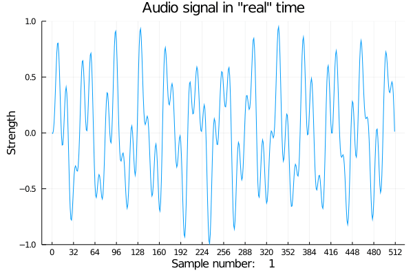
If only we could hear it.
using SampledSignals

# We're redefining the samples here just so the audio is a bit longer.
t2 = range(0.0, 40*pi, length = 20*N);
signal2 = 0.5*sin.(200*t2) + 0.2*sin.(445*t2) - 0.3*sin.(672*t2);

buf = SampledSignals.SampleBuf(signal2, 44100)
Honestly, this is incredibly impressive. It’s very cool to be able to write some very short code, manipulate a bunch of vectors, and then display that output in various ways. I can imagine that a Jupyter notebook running Julia like this would be very helpful for other, more serious blog posts.
For now, though, homework awaits.